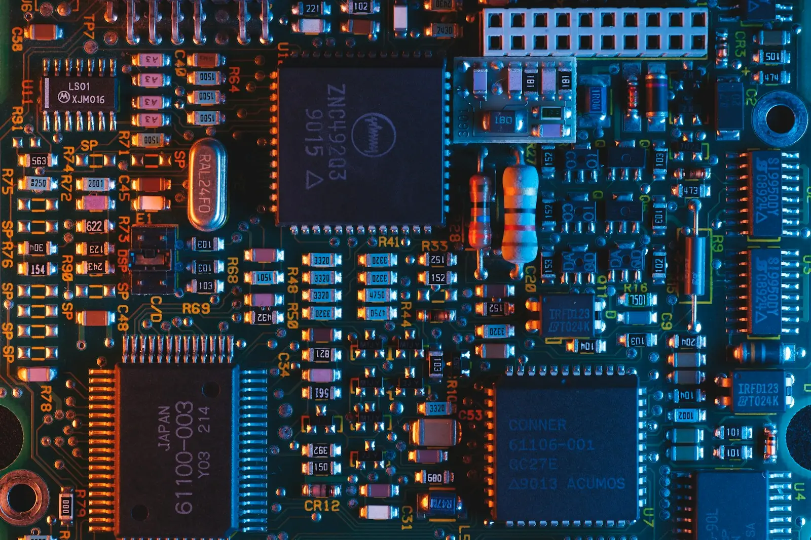
GPUs have become the default accelerator for plane-wave density functional theory, and Quantum ESPRESSO ships a mature GPU port that can cut wall-clock time dramatically on the right problem. But the speedup you actually see depends heavily on system size, the calculation type, and how the memory fits on the card. This guide explains what accelerates, why, and what to realistically expect before you commit GPU hours.
The QE GPU Port in Brief
Historically the GPU work lived in a separate QE-GPU tree, but modern Quantum ESPRESSO (since the 6.x series and consolidated in 7.x) integrates GPU support directly into the main codebase. The acceleration is built on CUDA Fortran and, more recently, OpenACC directives, compiled with the NVIDIA HPC SDK (nvfortran). The same pw.x, ph.x, and related binaries run on GPU when built with the right toolchain — you do not change your input files.
At runtime the GPU build offloads the heaviest numerical work to the device while keeping control flow and I/O on the CPU. The two dominant hotspots in a plane-wave SCF cycle are exactly the operations GPUs excel at: batched fast Fourier transforms and dense linear algebra. When your calculation spends most of its time in those two regions, the GPU port shines. When it does not, the benefit shrinks.
You can confirm GPU execution in the output header, which reports the detected devices, and by watching device utilization with nvidia-smi during a run.
What Actually Gets Accelerated
Understanding which parts of the SCF loop move to the GPU tells you which calculations benefit most.
FFTs: the Core Workhorse
Plane-wave DFT constantly transforms wavefunctions and the charge density between reciprocal space and real space. Applying the local potential, computing the density, and building the Hartree and exchange-correlation terms all rely on 3D FFTs. QE dispatches these to cuFFT, NVIDIA’s optimized FFT library. Because FFTs are memory-bandwidth bound and highly parallel, they map naturally onto GPU hardware, and this is often where the largest fraction of the speedup comes from.
Dense Linear Algebra: Diagonalization and Orthogonalization
Iterative eigensolvers (Davidson and the conjugate-gradient variants) repeatedly build and diagonalize the subspace Hamiltonian and orthogonalize trial wavefunctions. These operations are dominated by matrix-matrix products (ZGEMM) and dense diagonalization, which offload to cuBLAS and cuSOLVER. For systems with many electronic bands, this subspace work grows as roughly the cube of the number of bands and becomes a major cost — precisely the regime where GPU acceleration delivers the most.
What Stays on the CPU
Setup, symmetry analysis, force and stress bookkeeping, and file I/O remain largely on the host. Small serial sections do not accelerate and can become a relatively larger share of runtime once the heavy kernels speed up — a textbook case of Amdahl’s law. If the serial fraction is \(f\), the maximum speedup is \(1/f\):
$$ S_{\max} = \frac{1}{f + (1-f)/P} $$This is why tiny systems see modest gains even on powerful GPUs.
What Speedup Should You Expect
The honest answer is that speedups vary widely, from barely noticeable to an order of magnitude, depending on the problem. The numbers below are illustrative and representative of what plane-wave SCF workloads tend to show; they are not official guarantees.
| System size (atoms) | Typical CPU-node time | GPU-accelerated time | Illustrative speedup |
|---|---|---|---|
| ~10 (small cell) | 4 min | 3 min | ~1.3x |
| ~50 (surface slab) | 45 min | 12 min | ~3.7x |
| ~200 (supercell) | 6 h | 1.3 h | ~4.6x |
| ~500 (large defect) | 30 h | 5.5 h | ~5.5x |
The pattern is consistent: the larger the system, the better the GPU payoff. Small cells leave the device underutilized, and host-side overhead dominates. Large cells saturate the FFT and linear-algebra kernels, so the GPU runs closer to its peak throughput.
Other factors that move the needle:
- Calculation type. A plain SCF or
vc-relaxbenefits strongly. Hybrid functionals (EXX) are extremely FFT-heavy and can benefit even more, at high memory cost. Post-processing and NSCF band-structure runs benefit less per step. - Number of k-points. Many k-points give more independent work to batch, improving utilization on multi-GPU runs when combined with pool parallelization.
- Precision and pseudopotentials. Ultrasoft and PAW datasets add work on the dense FFT grid; norm-conserving sets are lighter.
Memory: the Real Constraint
The single most common reason a GPU run fails or underperforms is device memory. A GPU with 40-80 GB of HBM holds far less than a CPU node’s system RAM, and the wavefunctions, the charge density on the dense grid, and the subspace matrices must fit.
Memory footprint scales with the number of plane waves times the number of bands, plus the FFT grids. Practical consequences:
- If a system does not fit on one GPU, you must distribute across multiple GPUs using MPI, so each rank owns a slice of the bands and G-vectors.
- Hybrid functionals store additional quantities and can multiply memory demand several-fold; these often need multiple cards even for medium cells.
- Running one MPI rank per GPU is the common starting point. Oversubscribing ranks to a single GPU rarely helps and can exhaust memory.
If you hit out-of-memory errors, options include adding more GPUs, increasing pool or band distribution, or reducing ecutrho where physically justified after convergence testing. See our guide on parallelization in Quantum ESPRESSO for how the distribution levels interact.
When GPUs Help Most
GPUs are not a universal win. Use this quick decision framework.
flowchart TD
  A[DFT workload] --> B{System size}
  B -->|under ~30 atoms| C[CPU often better]
  B -->|over ~100 atoms| D{Fits in GPU memory?}
  D -->|Yes| E[GPU preferred]
  D -->|No| F{Can distribute<br/>across multi-GPU?}
  F -->|Yes| E
  F -->|No| C
  A --> G{Hybrid / long AIMD?}
  G -->|Yes| E
Strong GPU candidates:
- Large supercells, defect calculations, and surface slabs (roughly 100 atoms and up).
- Hybrid-functional (EXX) runs, which are dominated by FFTs.
- Long ab-initio molecular dynamics trajectories where per-step cost matters.
- Throughput workflows where you can pack independent runs across cards.
Weaker GPU candidates:
- Very small unit cells (a handful of atoms) where CPUs already finish quickly.
- Workloads dominated by serial setup or heavy I/O.
- Runs that do not fit in device memory and cannot be distributed cleanly.
For a deeper architectural comparison, see our companion piece comparing computational engines and the trade-offs between CPU and GPU execution.
How to Build and Run on GPU
With the NVIDIA HPC SDK available, a GPU-enabled build is configured roughly as follows:
./configure --with-cuda=$NVHPC_CUDA_HOME \
            --with-cuda-runtime=12.3 \
            --with-cuda-cc=80 \
            --enable-openmp
make -j pw
Here --with-cuda-cc is the target compute capability (for example 80 for A100, 90 for H100). Running a single-GPU SCF is unchanged from the CPU workflow:
mpirun -np 1 pw.x -inp scf.in > scf.out
For a multi-GPU node, launch one rank per device and let pool parallelization spread k-points:
mpirun -np 4 pw.x -npool 4 -inp scf.in > scf.out
Environment sanity checks before launching:
nvidia-smi— confirm devices are visibleecho $CUDA_VISIBLE_DEVICES— confirm the ranks see the right cards
Watch the timing summary at the end of the output: the fft, cegterg/ppcg, and h_psi timers tell you where the run spent its cycles and whether the GPU is doing the heavy lifting.
Common Pitfalls and Diagnostics
- No speedup on a small cell. Expected. Batch small jobs or move to a bigger system before judging the GPU.
- Out-of-memory crashes. Add GPUs and distribute; check the reported memory estimate near the top of the output.
- Poor multi-GPU scaling. Usually a pool/band mismatch or too few k-points to distribute. Tune
-npoolto your k-point count. - Numerical differences vs CPU. Small differences at the level of the SCF threshold are normal due to reduction ordering; they should vanish well within your convergence tolerance.
Always validate a new GPU build by reproducing a known CPU result for a small reference system before trusting large production runs. The official documentation and user forum at quantum-espresso.org track build requirements and version-specific GPU notes.
Multi-GPU Scaling in Practice
A single card takes you only so far. Once a system is large enough to benefit from GPUs, it is often large enough to need several of them, and scaling across devices introduces its own considerations.
One Rank Per GPU
The standard model is one MPI rank bound to one GPU. With four cards you launch four ranks, and each owns a slice of the bands and G-vectors. Binding matters: on a multi-socket node, a rank should use the GPU attached to its own NUMA domain, or the PCIe/NVLink traffic crossing sockets will erode the gains. Most cluster launchers and MPI implementations provide affinity flags to pin ranks to the right device.
Interconnect and Communication
As you add GPUs, inter-device communication starts to matter. The FFTs and diagonalization require data exchange between ranks, and on multi-node runs this crosses the network fabric. NVLink between cards on the same node is far faster than PCIe or Ethernet between nodes, so scaling within a node is usually more efficient than across nodes. This is why a densely connected multi-GPU node often outperforms the same number of GPUs spread thinly across many nodes.
Combining GPUs with Pools
For calculations with several k-points, pool parallelization pairs naturally with multiple GPUs: assign one pool per GPU so each device works on its own k-points with minimal cross-talk. Gamma-point runs, having a single k-point, instead rely on band and G-vector distribution across the cards, which communicates more and scales less perfectly.
Profiling to Confirm the Win
Never assume the GPU is being used well — measure it. Two cheap checks reveal most problems:
nvidia-smiduring the run. Sustained high utilization and memory occupancy mean the device is busy. Utilization bouncing near zero signals a host-bound bottleneck or a system too small to fill the GPU.- The QE timing summary. Compare the
fftand eigensolver timers against total wall time. If those dominate and total time dropped versus CPU, the offload is working. If setup or I/O now dominate, you have hit the serial-fraction ceiling.
If profiling shows the GPU idling, the fix is usually to grow the problem, batch independent jobs onto the same device, or revisit the rank-to-GPU mapping rather than to add more hardware.
Run it on Simatra
Simatra runs Quantum ESPRESSO on GPU-accelerated clusters using our GPU-Opt-V2 instances, delivering up to 5x faster convergence on large plane-wave workloads and supporting supercells up to roughly 2,000 atoms. You get both the Quantum ESPRESSO engine and our native KRONOS engine (a C++20, GPL-3.0 DFT code with CUDA, HIP, and Metal backends) — read more about both on our computational engines page. Skip the build headaches and start a free trial with $100 in credits at app.simatra.io.